Anomaly Detection in Time Series

Challenges

Anomaly Detection is particularly challenging when dealing with time series data.

• Time series data often suffer from missing values. It is important to handle these missing values adequately to not break the temporality of data and distort the anomaly detection algorithm.

• Companies scarcely annotate raw time series data. Because of this, there are often very few examples of true anomalies to work with.

• What is considered as “normal” changes over time. For example, the normal behavior of a piece of machinery will strongly evolve following a change of settings.

• What defines an outlier is extremely business driven, and subject to expert knowledge and specific rules.

• There are different types of anomalies.

Types of Anomalies

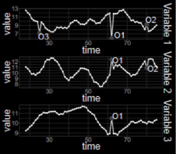
In literature, time series outliers are generally broken down into three types: Point Outliers, Contextual Outliers, and Collective Outliers.

• A Point Outlier is an individual data point that is anomalous with respect to the rest of the data.

• A Contextual Outlier is an individual data point that is anomalous within a specific context (often a time window), but not necessarily with respect to the entire dataset

• A Collective Outlier is a collection of successive data points that is anomalous with respect to the rest of the data.

These three different types of outliers can be either univariate or multivariate depending on whether there is one or multiple time-dependent variables that are affected at the timestamp of the anomaly.

Four Aspects to Consider

In order to choose the best approach to perform the anomaly detection, there are four aspects that should be considered:

• What is the business objective?

• What defines an outlier ? Which types of outliers are we trying to detect ? Are they univariate or multivariate ?

• Is there a strong dependence on time ? How important is the temporal order of observations ?

• What types of variables (endogenous, exogenous, business rules) do we want to use for modeling ?

Types of Models

The answers to these questions will guide the choice of the type of model that is best suited for the problem at hand. There are four main approaches to performing anomaly detection:

1 —  Supervised training of a binary classification model

While this tends to yield good performance thanks to the ability to train a model to classify normal vs anomalous, it requires having a large number of annotated anomalies, which is rare.

2— Predictive Confidence Level Approach

This approach is useful when we have a good understanding of the time series data, to the point that we are able to build a high-performance forecasting model (if you want to know more about forecasting models, you should check out this other article we wrote).

The idea is to predict the next observation thanks to the forecasting model, and compare the prediction to the actual value when it comes in. If the actual value is “too far” from the prediction, the point is considered anomalous (this distance can be either deterministic or probabilistic).

3— Majority Modeling

The goal of majority modeling is to model the distribution of normal data points. Anything too far from the distribution is an outlier. This can be done in two ways:

• Through a statistical profile — which in most cases leverages the temporal nature of data either with simple descriptors such as moving averages and standard deviation, or decompositions such as STL

• Through an unsupervised machine learning model — these ignore the temporal data structure and consider each data point independently

4— Discords Analysis

Mostly used for collective outliers, this approach measures similarity between subsequences defined by sliding windows and identifies discords as outliers (often through matrix-profiling).

Context & Goal

At Sia Partners, we had the opportunity to help one of our clients detect anomalies on a particular piece of equipment used throughout their industrial processes.

The goal was to create a system that would alert of potential anomalies (“candidates”), that would then be reviewed by experts who would determine the best course of action given the behavior of the equipment.

Data

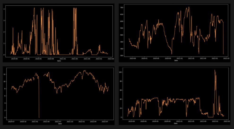
We had data for 16 different devices. Each device was equipped with sensors that measured 7 different signals (4 main and 3 secondary signals), with data points every 10 minutes. However, we decided to work with hourly data in order to reduce the amount of noise.

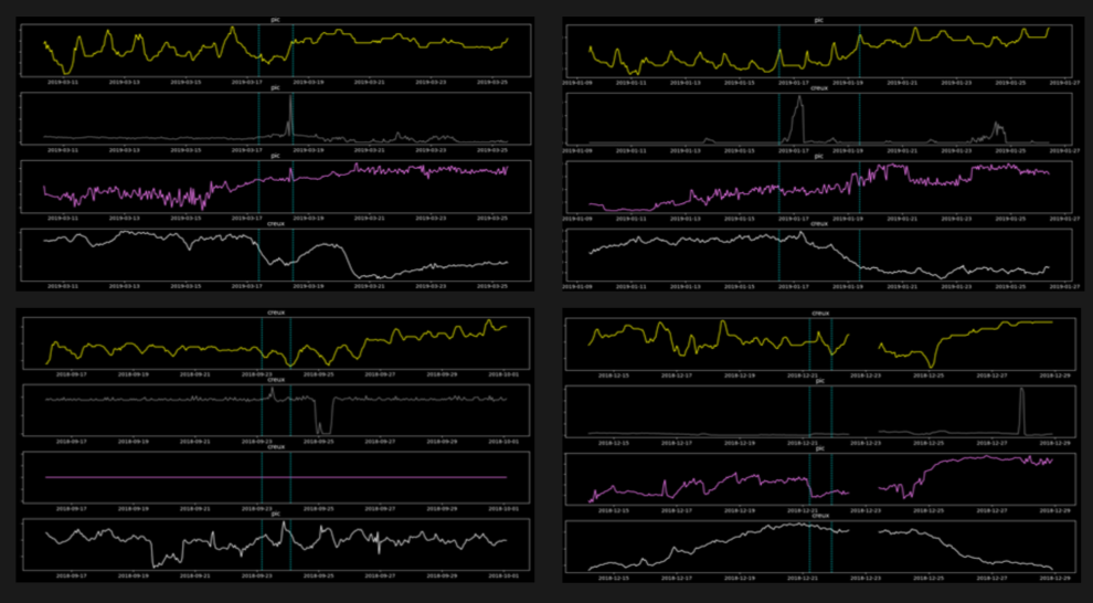
As demonstrated by the graphs below of the 4 main signals, the time series data was chaotic, with a high variance and range. Furthermore, we can see that there are different types of variations in the signals that last different amounts of time.

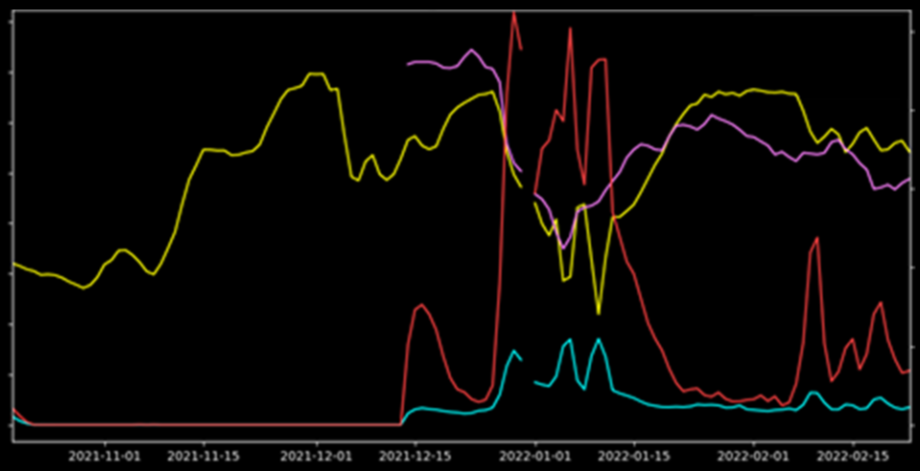
We did not have a significant annotated database of anomalous events we wanted to detect. Instead, all we had were a few dozen examples of behaviors that we wanted to be able to identify as being anomalous, such as the example below.

Scoping of anomaly detection task

Business Objective

The objective was to perform anomaly detection : as soon as an anomaly was raised, the company needed to be able to analyze the event and act upon it within the same day.

Outlier Definition

Even though anomalies could last in time, we were interested in detecting point or contextual outliers rather than collective outliers. There wasn’t a typical duration of an anomaly, so the aggregation of point outliers to lasting event-based outliers was to be handled through post-processing.

These outliers were multivariate and could span across 4 different time series.

Dependance on Time

It was unclear whether the observations were very time dependent: there was no clear tendency, seasonality, nor trend.

Modeling Variables

We were only interested in using the 7 endogenous variables from the sensors.

Modeling

Choice of Modeling approach

Given that we only had a few dozen labeled anomalies, performing supervised classification was out of the question. Discords Analysis was not appropriate either since we were not working on collective anomalies. Finally, the temporal dependency of the data was uncertain, and we did not have forecasting models for each of the four time series on which to detect outliers. Because of this, it did not make sense to try to build forecasting models to leverage a predictive confidence level approach.

Therefore, we chose to leverage different majority modeling techniques. We ended up implementing two different approaches:

• DBSCAN clustering-based anomaly detection
• Peak detection through a sliding-window based statistical profile

DBSCAN Clustering

Our first approach was to leverage the DBSCAN algorithm (Density-Based Spatial Clustering of Applications with Noise) in order to create clusters that would separate the normal and abnormal data points. DBSCAN presents a few advantages for multivariate anomaly detection:

• It is natively multivariate : it considers the value of the seven signals at each instant as points in a seven-dimensional vector space before grouping them into clusters.
• It does not require you to specify the number of clusters beforehand
• It does not assign each point to a cluster — all points too far from all the other clusters are assigned default cluster “-1”.

a — Preprocessing

But first, it was necessary to perform a few preprocessing steps on the data for it to be suited for DBSCAN:

• Min-max normalization to avoid issues due to the different order of magnitude of the signals for the Euclidean Distance used in DBSCAN
• Data imputation of the mean-value of the sensor to deal with missing data
• Mean-aggregation of the signals over the past 4 hours to compensate for the slight lack of synchronization between the variations of the 7 signals during anomalous events, because otherwise the DBSCAN algorithm does has no other was to take into account the temporal nature of the data

b — Implementation for anomaly detection

Given that each device is used in a different physical context, we applied preprocessing and clustering separately to each. Once these steps performed, we defined as anomaly candidates:

• All the data points not assigned to a cluster
• All the data points belonging to small clusters (< 5% of total).

The choice of the maximum distance between two clusters was very important to obtain one large cluster with over 90–95% of the data that represents the “normal” behavior of the device, and be confident that the small clusters & unassigned data should be studied as potential anomaly candidates.

In order to go from data point anomalies to lasting event anomalies, we then combined anomalous data points that belonged to the same cluster and had consecutive timestamps.

c — Limits

The implementation of this method is closer to post-hoc analysis : the cluster to which a given data point is assigned depends on all the data, whether it occurs before or after the given data point.

Nevertheless, it is possible to apply this method to a streaming anomaly-detection context: we simply need to assign each new data point to one of the existing clusters (or cluster -1). However, this assumes that the large clusters are stable enough over time and correctly model the “normal” behavior, which itself is stable over time. These conditions are not easy to satisfy, which is why we tried a second approach.

Peak detection through a sliding-window based statistical profile

The second approach we implemented was a peak and valley detection algorithm, that creates a moving-average statistical model for each signal during a sliding time window, and flags data points “too far” from the model as anomaly candidates.

This method presents a few advantages:

• It does not require any historical data for learning besides the data for the chosen size of the window
• It can be used in real-time in a streaming context to perform anomaly detection
• It does not require any specific pre-preprocessing

However, this method is natively univariate as it detects peaks and valleys in one specific time-series. We therefore need to apply it to each signal simultaneously before combining the outputs to detect multivariate anomalies.

Implementation for anomaly detection

This algorithm relies on three parameters:

• Window size — the number of data points we are going to use to create our moving-average model, and determine if the following data point is a peak or valley.

• Difference threshold — the number of standard-deviations away from the moving window average that a data point needs to be in order to be considered a peak or valley.

• Relative importance of peaks — the influence (between 0 and 1) of a peak or valley on the detection of a consecutive peak or valley. An influence of 1 means that two consecutive peaks will be considered as one, and an influence of 0 would detect all peaks independently.

We performed grid-search to find the optimal parameters for each signal, which varied given signal specificities but were generally around a 35 hour window size, a difference threshold of 3, and a relative importance of 0.8.

After detecting peaks and valleys on each of the 4 main signals belonging to a device, we then combined these peaks and valleys to create multivariate events:

• If they were less than one day apart
• If there was a peak or valley in at least 3 of the 4 signals.

We then continued combining multivariate events if they were less than a day apart in order to capture lasting anomalies.

Results

We did not have a large annotated dataset to measure model performance. We were mostly in an unsupervised context, except for the dozen available examples annotated by subject-matter experts. Therefore, our goal was to:

• Maximize the recall on our dozen available anomaly examples (percentage of our dozen anomalies that were correctly detected by the algorithm)

• All the while minimizing the number of potential candidates flagged in order to increase precision (keeping in mind that there were many true positives beyond the dozen annotations, so it was impossible to compute the actual precision)

It was important to try to keep a generic approach that would fulfill both these goals and visually inspect the relevance of the flagged candidates in order to avoid overfitting on the dozen annotated anomalies.

DBSCAN Clustering

Let’s first look at the results of our DBSCAN Clustering approach.

Overall, this approach was able to obtain 66% recall, and identify 165 other potential anomaly candidates.

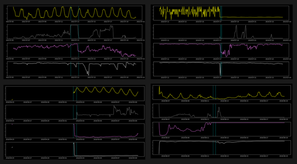
Visual observation of the 165 candidates enabled us to identify four types of situations caught by the model:

1. True positives that were not annotated by the subject-matter experts
2. Very short events detected slightly after an actual event, due to the 4 hour averaging
3. False positives due to the sudden change from missing data to actual data
4. False positives that are more difficult to explain

Peak detection through a sliding-window based statistical profile

The peak detection approach was more sensitive to anomalies: it reached 100% recall on our dozen examples, but identified over 1200 potential candidates.

We therefore implemented additional post-processing rules to reduce the number of candidates. These were able to combine successive peaks and valleys, filter out very short anomalies that were due to maintenance, and implement additional use-case specific rules.

Thanks to these additional steps, we were able to reduce the number of candidates to 276, while maintaining an 86% recall.

Visual observation of the candidates also enabled us to identify four types of situations caught by this model:

1. True positives that were not annotated by the subject-matter experts
2. Long events lasting a few days
3. False positives due to a missing signal
4. False positives that are more difficult to explain

By comparing the results of both approaches, it seems that the peak-detection method has a higher performance potential thanks to its ability to be combined with expert rules, an advantage of time-series based approaches compared to clustering that relies on an abstract 7-dimensional vector space.

However, there is only a 58% overlap between candidates from both methods. This indicates that the two approaches are complementary!

The next step for our client was therefore to apply both approaches to identify potential candidates, and begin creating an annotated dataset that could later be used to train a supervised classification model.

This use case demonstrates a challenging anomaly detection task for time series in a real-world situation, where forecasting models were not the appropriate method. Finding the right approach based on clients’ business objectives, outlier types, and data was key to cracking their problem and developing a valuable anomaly detection solution.

If you would like to know more about our Time Series, Anomaly Detection, or Data Science & AI expertise, please do not hesitate to contact us.