Data driven customer segmentation: Deep dive on segmentation and interpretation

A. Processing and segmentation algorithms

     1. Preprocessing

Pre-processing is a purely technical - but necessary- step for machine learning algorithms and especially clustering. First of all, it is necessary to one-hot encode categorical variables to avoid correlations because clustering algorithms are based on distance calculations and only work only numerical variables. The function used for this task is get_dummies from Pandas library with the option drop_first = True. 

Besides, in order to not bias the clustering by overweighting a variable with a different scale, it is also necessary to standardize the numerical variables. For this specific task, we use the predefined MinMaxScaler from Scikit-Learn library.

Last but not least, a major step of the pre-processing consists in checking the correlations between variables and processing. Two choices are possible: Either to delete the correlated variables to avoid redundant information or perform a Principal component analysis (PCA). Regarding the first method, we use a correlation threshold of 0.9 and keep the more relevant variable in a business sense.

     2. PCA

Principal component analysis aims to reduce the dimensions of features. It seeks to find a new orthonormal basis in which we can represent the data in a much simpler way such that the data’s variance along these new axes is maximized.

This analysis is optional, but PCA is particularly useful when the variables are highly correlated and numerous. In this case, it reduces the original variables into a smaller set of variables while preserving as much of the data's variation as possible from the original dataset. For implementation, we commonly use the scikit learn library as it proposes the decomposition.PCA class.

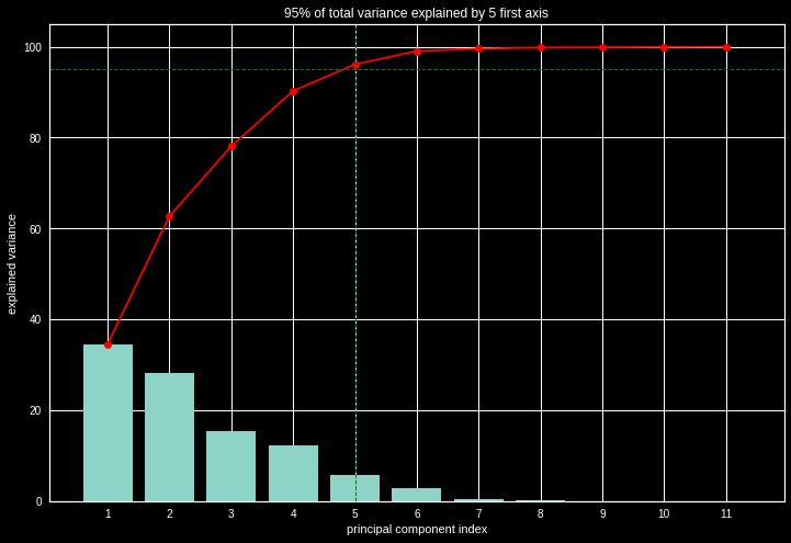
To determine the number of optimal components, one of the methods resides in looking at the cumulative sum of the eigenvalue inertias and taking the k axes that keep 95% of the inertia.

     3. Kmeans

K-means clustering is one of the most widely used unsupervised segmentation algorithms. It is an exploratory method that relies on heuristics. It is an iterative method that searches for the clusters’ centroids in order to partition the observations into K clusters.

After randomly initializing the centroids, K-Means allocates every data point to the nearest cluster, while keeping the centroids as small as possible by replacing each centroid according to the descriptors’ average within its group. It then performs iterative calculations by repeating the same step a number of times until convergence. To implement K-means, the number of clusters is defined beforehand by the user after using the elbow method and the silhouette coefficient to find the optimal number.

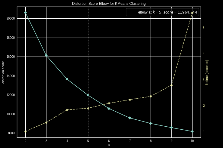
The elbow method is a visual method that consists in calculating the variance of the different volumes of clusters considered, then plotting the obtained variances on a graph that will resemble the shape of an elbow. The optimal number of clusters is then identified as the point representing the tip of the elbow, i.e. the point corresponding to the number of clusters from which the variance does not decrease significantly.

For example, with Kmeans implemented within the scikit learn library, it is possible to use the yellowbrick package then KElbowVisualizer to obtain the following graph showing the inertia. Here, the recommended number of clusters = 6.

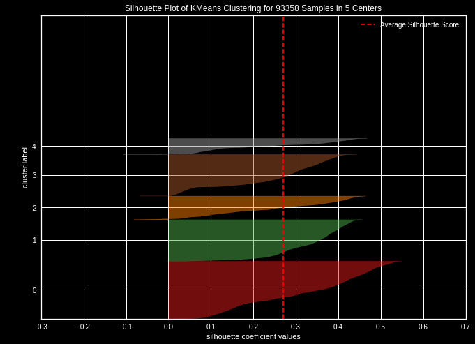
Alternatively, we can use the silhouette coefficient which represents the partition quality of a data set in automatic classification. For each point, its silhouette coefficient corresponds to the difference between the average distance to points within the same group (cohesion) and the average distance to points in other neighboring groups (separation). If this score is negative, the point is on average closer to the neighboring group than to its own, and is therefore, poorly ranked. Conversely, if it is positive, the point is on average closer to its group than to the neighboring group meaning that it is well ranked.

The silhouette coefficient itself is the average of the silhouette coefficient of all points. A predefined implementation is available in scikit learn library in the category metrics / silhouette_score 

     4. ACH

Agglomerative hierarchical clustering aims at dividing the points into k homogeneous and compact groups or clusters. The main idea resides in calculating the dissimilarity between observations.

The approach is different from Kmeans since the starting idea is to consider that each point of the dataset is a centroid. Then, each centroid is grouped with its closest neighboring centroid according to a defined distance (by default Euclidean distance). Afterwards, we calculate the new centroids representing the gravity centers of the newly created clusters. The operation is repeated until a single cluster is obtained or the observations are partitioned according to a number of clusters defined beforehand.

However, the use of the ACH can lead to memory problems because of 2 to 2 distance calculations which enhances complexity. 

First, it is necessary to run the algorithm without determining the number of clusters. This means that each point is considered as a cluster. The display of the dendrogram provides us first insights on the optimal number of clusters. We can also apply the elbow method or the silhouette coefficient.

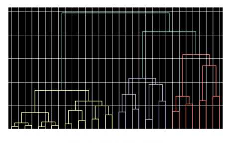
The dendrogram allows to visualize the successive groupings until a unique cluster is obtained. It is often relevant to choose the partitioning corresponding to the largest jump between two consecutive clusters. The number of clusters then corresponds to the number of junctions kept.

In the example below, the horizontal cut corresponds to the two red lines. There are 3 vertical lines crossed by the cut. We deduce that the optimal number of clusters is 3.

For implementation purposes, we can use  scipy.cluster.hierarchy to plot the dendrogram.

     4. Clustering methods comparison and use cases

In the table below, we can find both advantages and inconveniences for both clustering methods.

Kmeans

Advantages :

• Spherical clusters (all cluster points have the same variance)
• Low computational cost
• Suitable for a large dataset and provides a deterministic assignment.

Disadvantages: 

• Inconsistencies between 2 runs due to random initialization
• Sensitive to outliers
• Does not allow to non-convex groups identification

ACH

Advantages :

• More accurate
• Dendrogram highlights the clusters’ dispersion

Disadvantages: 

• Not suitable for large datasets (2 to 2 distance calculation for each point

However, we can combine these two methods for more robustness. Two approaches can be implemented depending on the order:

• ACH before K-means: allow reallocation of boundary points between 2 clusters in the dendrogram. 
• K-means before ACH: if the number of observations N is high, use a large number of clusters K for the K-means (to avoid memory problems). 

B. Interpreting segmentation results

After applying clustering to our dataset,  we end up, for each of our clients, with a label referring to the cluster to which it has been assigned. As a second step, we seek to describe these segments more precisely. In this context, two methods can be considered for results interpretation: 

1. K-means discriminating variables Analysis
2. Decision tree Visualization 

Then we will try to identify the issues of each segment and validate the key moments:

3. Interpretation of the time window for which the K-Means is relevant 
4. Visualization of clusters’ evolution over time and customers’ tendency to move from one cluster to another using Markov Chains (transition matrix)

This last step is essential in the implementation of a data-driven activation strategy in order to identify the objective elements that will feed the strategy.

     1. Analysis of discriminating features and interpretation

This analysis relies on average calculations for each feature per cluster. We can visualize the impact of these variables on each cluster with the "radar plot", showing the value of the features for each cluster.

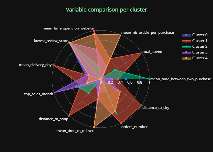
Radar graphs facilitate the interpretation of the segmentation, allowing us to easily deduce an "ID card" of the different clusters which makes it easier for business to understand these outputs.

The advantage of this first interpretation method is that it is solely based on the K-means outputs, thus ensuring to get business rules that correspond exactly to what is visible through the K-Means clustering.

     2. Decision trees

Alternatively, we can visualize outputs via  "Decision Tree" type classifiers by focusing on the variables that seem to best separate the different clusters. 

You can use the dtreeviz library to plot the output of a classification.

The goal here is to obtain simple and easily interpretable business rules to distinguish clusters even if it means discarding statistical reality.

     3. Analysis of K-means temporal stability 

In order to establish the robustness of the customer segmentation algorithm, we need to test its stability over time, and see when customers change clusters. To do so, we need to recalculate all the features according to a given period (2 months), and look at the algorithm evolution over time using the ARI score.

ARI stands for Adjusted Rand Index which expresses the probability that two different customers belong to the same group in two different segmentations.

The ARI is useful for the interpretation of a customer base characterized by a high frequency of purchase as it allows to know when a customer will change segment.  However, the duration is highly sector-dependent.

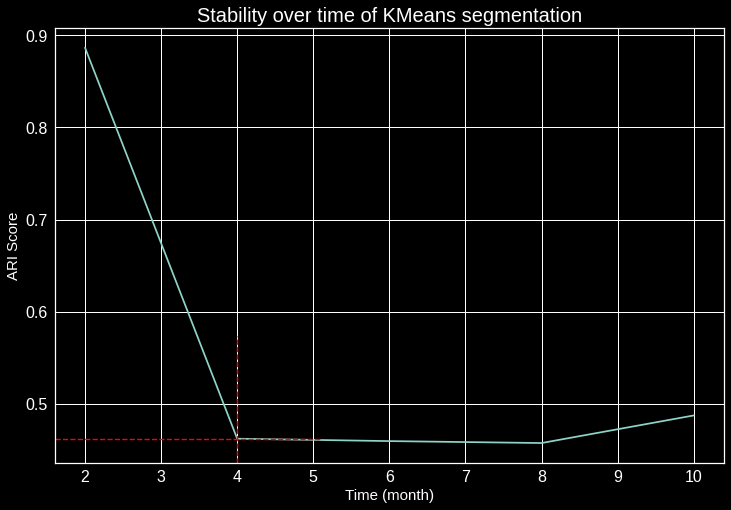
This graph shows that the inflection of the ARI score starts as early as the 2nd month, we also notice a strong inflection after 4 months on the initial customers. Reviewing the segmentation program every 4 months is thus highly recommended.

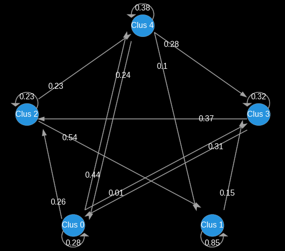
     4. Markov Chain - Transition matrix

In order to identify marketing issues for each cluster, we saw that it is important to monitor and visualize the segmentation’s temporal stability. We will now go through the virtuous flows: Either by simply cross-segmentation over two successive periods or by using Markov Chains to calculate and plot the probability of a customer to move from cluster A to cluster B. This technique allows us to identify the different paths in the long run, but can only be visually represented in 2 dimensions. It will therefore be necessary to adopt both types of approaches.

In the example below representing our 5 clusters, we can see the clusters’ evolution every 2 months:

Conclusion

A successful marketing segmentation needs to be interpretable. One must obviously master data science methodologies, but also not lose sight of the business objective. This means taking business constraints into account in the algorithms, ensuring interpretability and giving the business stakeholders the means to activate the segmentation by precisely qualifying and analyzing customer behavior.  

After designing and implementing a data-driven segmentation, we must be able to identify and identify the characteristics and challenges of the output segments and  key moments of their life cycle. From these analyses, marketing teams will be able to build personas and implement a dedicated marketing strategy per segment based on an in-depth knowledge of the customer journey and its specificities.