Auto encoder and SHAP values: Detection and interpretation
Anomaly detection is the process of identifying irregular patterns in data. Its use is widespread, from fraud detection to predictive maintenance or churn detection. As a result, a whole branch of machine learning algorithms has been developed around these topics.
Most machine learning anomaly detection algorithms, such as Isolation Forest, Local Outlier Factor, or Autoencoder, generate a probability score for each data point of being an anomaly. The distinction between normal values and anomalies is then made most of the time by choosing a threshold.
These algorithms can be very efficient, and save experts precious time for inspecting a whole dataset. However, there is a major drawback of using machine learning algorithms: Most of them work as a black box, and give no information on why observation is considered an outlier. In a business context, the trust of the experts and companies in machine learning algorithms relies heavily on their capacities to explain their outputs.
We will here introduce and illustrate a method described in the preprint Explaining Anomalies Detected by Autoencoders Using SHAP, from Negev University, Israel [1]. It relies on the use of autoencoders, and of a framework, we will present, SHAP.
What is an autoencoder, and how to use it to detect anomalies ?
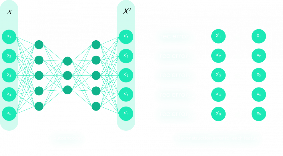
Autoencoders are a type of artificial neural network introduced in the 1980s to address dimensionality reduction challenges. An autoencoder aims to learn representation for input data and tries to produce target values equal to its inputs: It represents the data in a lower dimensionality, in a space called latent space, which acts like a bottleneck (action of encoding) and reconstructs the data into the original dimensionality (action of decoding). Based on the input, the autoencoder builds the latent space such that the autoencoder’s output is similar to the input and the embedded model created in encoding represents normal instances well. In contrast, anomalies are not reconstructed well and have a high amount of reconstruction error, so in the process of encoding and decoding the instances, the anomalies are discovered.
As a classic neural network, the autoencoder adjusts its weights using gradient descent, in order to minimize a function. In a supervised classification neural network, this function is the distance/error between predictions and labels. In the case of autoencoder, the error is the reconstruction error, which measures the differences between the original input and the reconstruction.
What are SHAP values ?
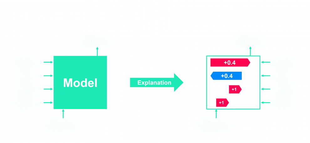
As said in the introduction, Machine learning algorithms have a major drawback: The predictions are uninterpretable. They work as a black box, and not being able to understand the results produced does not help the adoption of these models in a lot of sectors, where causes are often more important than results themselves. A type of tool has therefore been developed to allow understanding models decisions. The SHAP Value is a great tool among others like LIME, DeepLIFT, InterpretML, or ELI5 to explain the results of a machine learning model.
This tool comes from game theory: Lloyd Shapley found a solution concept in 1953, in order to calculate the contribution of each player in a cooperative game. We define the following variables:
- the game has P players
- S is a subset of the P players
- v(X) as the cumulated value of the set of X players.
- i is a player that is not part of the S players.
The value of the group S + i is, therefore, v(S+ i). If we want to calculate the value of i, v(i) = v(S∪i) — v(S). To have a good estimate of the marginal value, we take the average of the contribution over the possible different permutations of players.
This method to see the contribution of the features is adapted to based tree models, in which variables enter the machine learning model sequentially in the trees of the model. And given the number of trees and branches, we should observe all feature's permutations. For other models than trees, SHAP proposes a variant of the main algorithm, adapted to the model specificities, such as GradientExplainer, LinearExplainer, DeepExplainer…
We will use in the next part the SHAP (Shapley Additive exPlanations) implementation from [2].
Because we are using autoencoders, a deep learning model, we will use DeepExplainer, based on the publication Learning Important Features Through Propagating Activation Differences
How to interpret anomalies using Autoencoder and SHAP
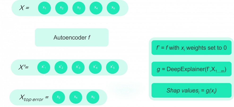
First, we use a simple autoencoder that we built using keras.
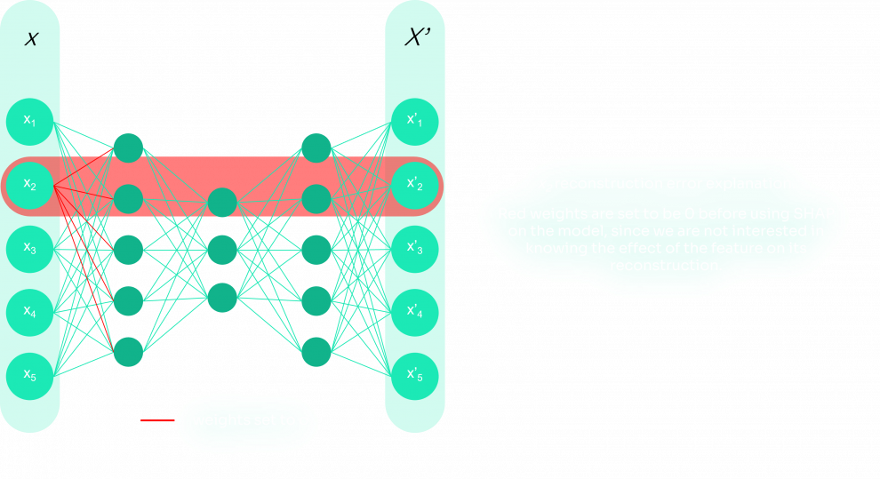
The autoencoder to use can have a different structure. However, it is important to keep the first hidden layer called hid_layer1, since we will then modify the weights of this layer.
Then, we use this autoencoder to determine the reconstruction error per observation, and for each observation, we order the features by their reconstruction error:
And we select the m features that have the highest error. We choose m such that the sum of the feature errors accounts for a good part of the total reconstruction error (80% for instance).
These features are stored in topMfeatures. Next, for each feature in topMfeatures, we will use SHAP to determine which features contribute to its reconstruction error, and which features offset the reconstruction error.
To do so, we start by eliminating the weights associated with the inspected feature in the model, since we are not interested in knowing the effect of the feature on its reconstruction. Then, we use the SHAP DeepExplainer to obtain the SHAP values, and we store them. Below is the algorithm for this process:
weights elimination for the current feature
algorithm representation
To test this method, we used a Credit Card Fraud Detection dataset from Kaggle [4]. This dataset contains transactions made by credit cards from two days in September 2013 by European cardholders. It contains 30 numerical input variables which are the result of a PCA transformation. Due to confidentiality issues, we do not have background information about the data. Features V1, V2, … V28 is the principal components obtained with PCA, and the only features which have not been transformed with PCA are ‘Time’ and ‘Amount’.
First, we have to distinguish the anomalies from the normal data points. Traditionally, we would choose a threshold that limits the number of false positives and true negatives as much as possible. But we could also use a modified Z-score value to identify outliers, as presented in [4]. This is the method we will use.
Using this method, we found 2,223 outliers in a total of 84,807 transactions.
Below is an example of the result we obtained for a detected anomaly: In red are the values contributing to the anomaly, in blue are the values offsetting the anomaly. We used the force_plot method of SHAP to obtain the plot.
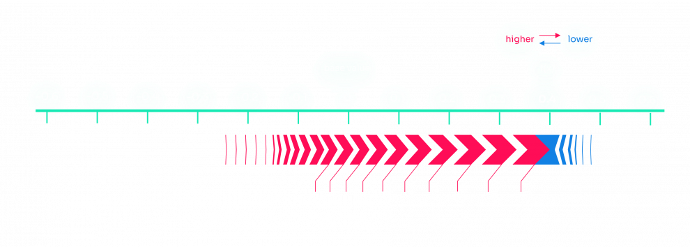
Unfortunately, since we don’t have an explanation of what each feature means, we can’t interpret the results we got. However, in a business use case, it is noted in [1] that the feedback obtained from the domain experts about the explanations for the anomalies was positive.
At Sia Partners, we have worked and are working on several anomaly detection missions, such as detection of anomalies in customer data, in chlorine concentration measurements, etc…
We are also working on the design, deployment, and management of AI-powered applications, through our Heka ecosystem. If you want to know more about our AI solutions, check out our Heka website.