Customer churn prediction with Data Science

In the field of marketing, scoring is a technique that enables one to assign a score to a customer or a prospect. The corresponding score generally reflects the probability that a customer or prospect will answer a marketing solicitation. 

 Many scoring techniques can be used in marketing, for different contexts, purposes and available data (lead scoring, risk scoring, predictive scoring, etc.) For example, predictive scoring can be used to identify customers at high risk of attrition. This is called churn prediction. 

Our use case ‍? 

In order to present a complete approach of churn prediction, we will use data from the music streaming service KKBOX in order to build a predictive model. Please note that for KKBOX a churn customer is a customer who has not renewed their subscription within 30 days of the expiration date of their last subscription. 

4 data files from KKBOX will be used: 

The approach for this use case will begin with an exploratory analysis (data quality & exploration), before preparing the dataset (pre-processing, feature engineering) for the modeling (training, testing & validation of the models) and interpretation of the results. 

A. Data Quality 

Data quality measure data’s status based on factors such as accuracy, completeness, consistency, reliability and whether it is up to date or not. 

This step is essential in any Data project as it prevents any potential gaps and errors. These issues need to be resolved before further analyzing the data or starting modeling efforts. 

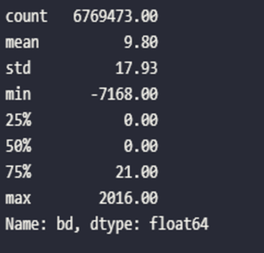
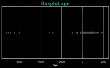
In our case, if we look for instance at customer’s age, we can find multiple outliers (ages from -7168 to 2016 years old). We will use a Machine Learning method to rectify this data.

Detecting outliers can be achieved through several methods : 

• Histograms. Outliers are often easy to spot in histograms. 

• Interquartile range. The interquartile range (IQR) tells you the range of the middle half of your dataset. You can use the IQR to create “fences” around your data and then define outliers as any values that fall outside those fences. 

• Z-score. Z-score indicates how far the data point is from the mean considering the standard deviation. All the observations whose z-score is greater than three times standard deviation i.e. z > 3, are considered as outliers. 

B. Data exploration 

Data exploration helps in making better decisions with features and model selection. Often, certain types of ML/DL algorithms are more suitable for a certain type of data.  

With a good idea of the data, we can better prepare the data for modeling. 

For this part we can BI tools (such as Tableau and PowerBI) as they enable us to produce quickly multiple graphs about the data. 

It is also possible to make data exploration with coding, as explained in this medium article.  

A. Data transformation 

This step transforms the data into a format that can be easily processed by a model. 

• Multicollinearity occurs when two or more variables are strongly correlated. It leads to bad results for some models, such as linear models. 

• Normalizing the features makes it possible to decorrelate them. Depending on the use case, the aggregation can be done by the mean, median, sum, etc. 

import seaborn as sns 

import matplotlib.pyplot as plt 

import numpy as np 

corr = customers.corr() 

mask = np.zeros_like(corr) 

mask[np.triu_indices_from(mask)]= True 

fig, ax = plt.subplots(figsize=(42,20)) 

ax = sns.heatmap(corr, vmin=-1, vmax=1, fmt=".2f", annot_kws={'size':8}, mask=mask) 

plt.title(f"Heatmap of linear correlations\n", fontdict=font_title) 

plt.show() 

B. Preprocessing 

Depending on the model you want to use (see part III), once the useful variables have been selected and the file prepared, it is essential to preprocess the data. 

For instance, if the model considers only  numeric variables, categorical variables must be transformed into numerical (i.e., encoding). In our use case we will use one-hot encoding.  

Please note that One-hot-encoding is a powerful technique to treat categorical data, but it can lead to an increase of dimensionality, sparsity and overfitting. It is important to use it cautiously and consider other methods such as ordinal encoding or binary encoding: 

city = pd.get_dummies(X.city, prefix='city') 

X = X.join(city) 

For numeric variables, it may be required to standardize them so as not to bias the algorithm if two variables are not on the same scale. You can use the MinMaxScaler() preprocessor.  

from sklearn.preprocessing import MinMaxScaler 

scaler = MinMaxScaler() 

X[numerical_features] = scaler.fit_transform(X[numerical_features]) 

C. Dealing with Unbalanced Datasets 

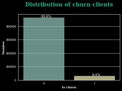
It regularly happens to have unbalanced dataset  (in our case 93% non-churn vs 7% churn). The risk is that the model simply predicts all or most of the points as the majority class because the data is biased. Some models, such as linear models, are not efficient in this type of situation. 

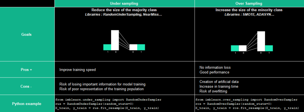
For the training phase, rebalancing the data is required, while test data shouldn’t be modified. Please note that some models include data rebalancing. 

There are two approaches to rebalancing data: 

For deep dive:  

• Handling Imbalanced Dataset With UndersamplingTechnique. Its Pros and Cons! 

• Handling Imbalanced Datasets With Oversampling Techniques. It’s Pros & Cons. 

Model training 

In order to predict churn customers, we trained several types of classification algorithms: XGBoost, Random Forest, SVM and Logistic Regression. The final model will be selected according to the results and the use case objectives. 

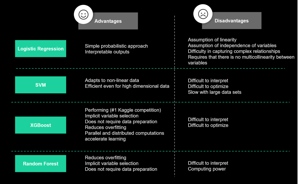
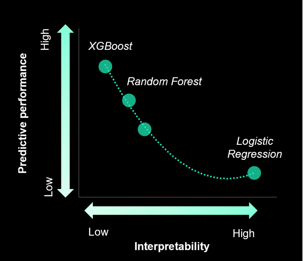
Models can be optimized by varying their hyperparameters. In our use case, these were optimized from a k-fold cross-validation. 

There are two methods to achieve this hyperparameter optimization: 

from sklearn.model_selection import  RandomizedSearchCV, GridSearchCV 

xgb = xgb.XGBClassifier() 

# hyperparamètres 

params = { "colsample_bytree": np.arange(0.5, 1.0, 0.1), 

           "gamma": uniform(0, 0.5), 

           "learning_rate": [0.01, 0.1, 0.2, 0.3], # default 0.1  

           "max_depth": randint(3, 7), # default 3 

           "n_estimators": randint(100, 200), # default 100 

           "subsample": np.arange(0.5, 1.0, 0.1), 

           "min_child_weight" : range(1,6,2)} 

# Randomized Search 

search = RandomizedSearchCV(xgb,  

                            param_distributions=params,  

                            random_state=42,  

                            n_iter=20,  

                            cv=5,  

                            verbose=3,  

                            n_jobs=1, 

                            scoring='accuracy',  

                            return_train_score=True) 

# Grid Search 

search = GridSearchCV(xgb,  

                            param_distributions=params,  

                            random_state=42,  

                            n_iter=20,  

                            cv=5,  

                            verbose=3,  

                            n_jobs=1, 

                            scoring='accuracy',  

                            return_train_score=True) 

search_result = search.fit(X_train, y_train) 

print("Best parameters:", search_result.best_params_) 

print("Best score: ", search.best_score_) 

xgb = search_result.best_estimator_ 

To learn more about hyperparameter optimization, we recommend this medium article.  

Choosing the metric to evaluate the model will depend on the use case. In our case, we seek to maximize the recall metric. Indeed, for our Marketing use case, the goal is to reduce False Negative (FN) as much as possible. which represent churned customers but were not predicted as such by the model. 

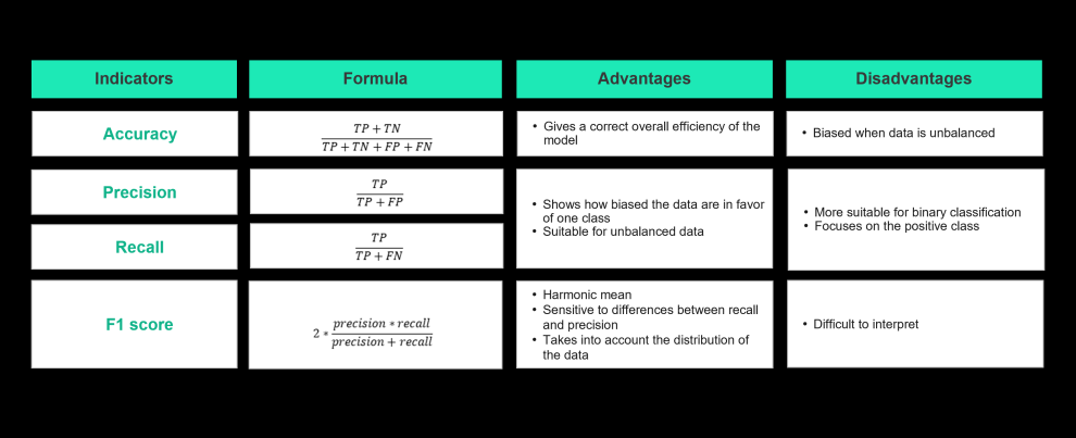
To learn more about metrics, we recommend this medium article.  

Model performance 

The results presented below come from an XGBoost model (which was the best model for our use case). 

The model produces for each customer a score corresponding to its churn probability. These customers are qualified as churner/non-churner according to a threshold which will be defined according to business needs (note: the threshold is by default at 0.5) 

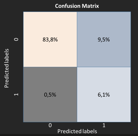
For a given threshold it is possible to produce a confusion matrix in order to quickly measure the results and the model’s types of errors. 

Here, the confusion matrix produces the following measurements on the model: 

• 84% (out of 93%) of non-churners  

• 6.1% (out of 7%) of churners. 

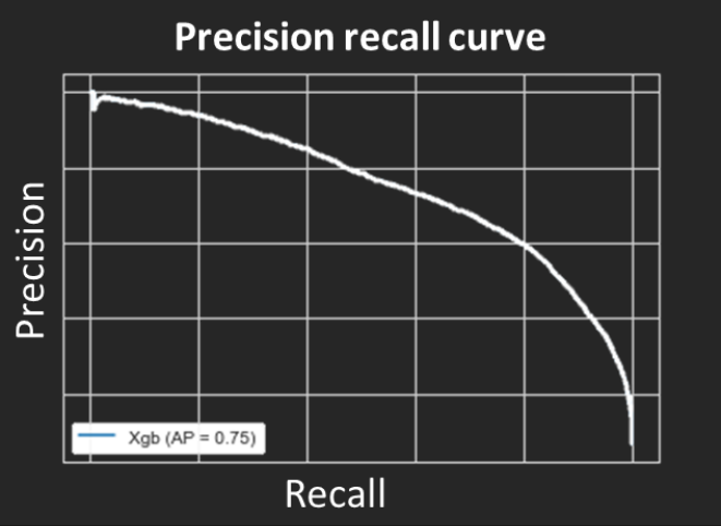
The recall metric is 93% but the precision metric is 39%. In that case, the model predicts more churners customers than there are. There is a trade-off between these two metrics. Depending on what you want to achieve, the probability threshold must be adapted in order to obtain an optimal result of your use case. When we have an unbalanced dataset, the precision-recall curve allows you to visualize the result of these two metrics for all the probability thresholds. 

It is quite important in marketing to be able to explain, globally and locally (i.e. at a client level) how a prediction was made. Knowing which feature contributed and how much will allow you to better understand your model and reassure the end user by giving visibility on each client score.  

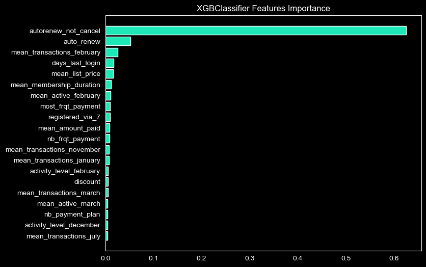
Our XGBoost model allows us to obtain the most important variables that permitted to make a prediction.  

In our case, these variables are: 

• autorenew_not_cancel (automatically renewing all subscriptions and canceling none) 

• auto_renew (automatically renewing all subscriptions) 

• mean_transactions_february (average amount of transactions in February) 

These key variables are to be compared with the business - for example, trying to understand why the month of February has more weight in the prediction than the other months (i.e. was there a particular action on the KKBOX side in February?) 

fig, ax = plt.subplots(figsize=(8,6)) 

ax.grid(False) 

sorted_idx = xgb.feature_importances_.argsort()[-20:] 

plt.barh(X_train.columns[sorted_idx], xgb.feature_importances_[sorted_idx], color = "#1DE9B6") 

plt.title("XGBClassifier Features Importance") 

Explain the model prediction 

This part will be covered in a following article where we will interpret the model with the SHAP library (Python library based on optimal Shapley values in game theory). 

Note: Shapley values calculate the importance of a variable by comparing what a model predicts with and without this variable (taking order into account). This approach makes it possible to explain the results of Machine Learning models by estimating the contribution of each variable. 

The SHAP library offers a global interpretation, that permits us to show to what extent each predictor contributes and the positive or negative relationship of each independent variable with the dependent variable. It also offers a local interpretation, that permits us to explain why in each individual case we get this prediction and the predictors’ contributions. 

This article has showcased the development of a scoring model for the prediction of customer churn. 

We will go further in the analysis of customer churn with the usage of the SHAP & LIME library to better understand the positive and negative relationship of the contribution at several scales (global/local) in a second article.